KINGSTON, R.I. – Sept. 1, 2022 – The University of Rhode Island Theatre Department’s upcoming season will transport audiences from the darkest edges of the city where “dreamers, dealers and desperadoes” roam, to a 17th century London flat and the meetings of lovers and spies, to the trials of a young Black actress in 1930s Hollywood, and leave them deep “Into the Woods” listening to Sondheim’s Tony Award-winning music.
Always a diverse lineup, URI’s season will bring to the Robert E. Will Theatre stage thought-provoking and, at times, laugh-out-loud funny contemporary works by award-winning playwrights – that are equally compelling for audiences and theatre students, on stage and behind it.
“Each of our four productions has such an exciting and unique perspective,” says David Howard, chair of the Theatre Department. “We have a lot of new plays that are being produced and we will have a lot of new guest artists joining us.”
The season opens Oct. 13 with Naomi Iizuka’s 1997 “Polaroid Stories,” which mixes classical mythology and real-life stories of drugs, violence, and money from kids living on the streets in society’s shadows. Howard calls it “a very modern and edgy piece that students are really excited about.”
The play, directed by guest artist Patrick Saunders, introduces street-wise kids whose characters are adapted from Ovid’s “Metamorphoses,” an epic poem of mythic heroes and monsters. While the play has a mean-streets feel of graffiti, garbage and concrete, scenic designer James Horban is exploring a setting that recognizes the play’s abstract bridging of stories tied together through mythology.
“‘Polaroid Stories’ is the type of play that can be produced in a variety of ways,” he said. “It’s less strict about dictating the setting. From a design perspective, what was really important to me in choosing our season was having room to grow on the spectrum of realistic sets or something more open ended.”
For the season’s second play – Liz Duffy Adams’ hysterical and historical “Or,” which opens Dec. 8 – the Theatre Department is trying something a little different. “Or,” will be the annual student-run, full-length production, where students fill every job, from actor to director to designer. Instead of being produced on the season’s fringes, the play will be part of the main productions, allowing students to throw in all the bells and whistles available. While students have an equal say in choosing each season’s lineup, “Or,” was selected by senior Sarah Taylor, who will direct the play.
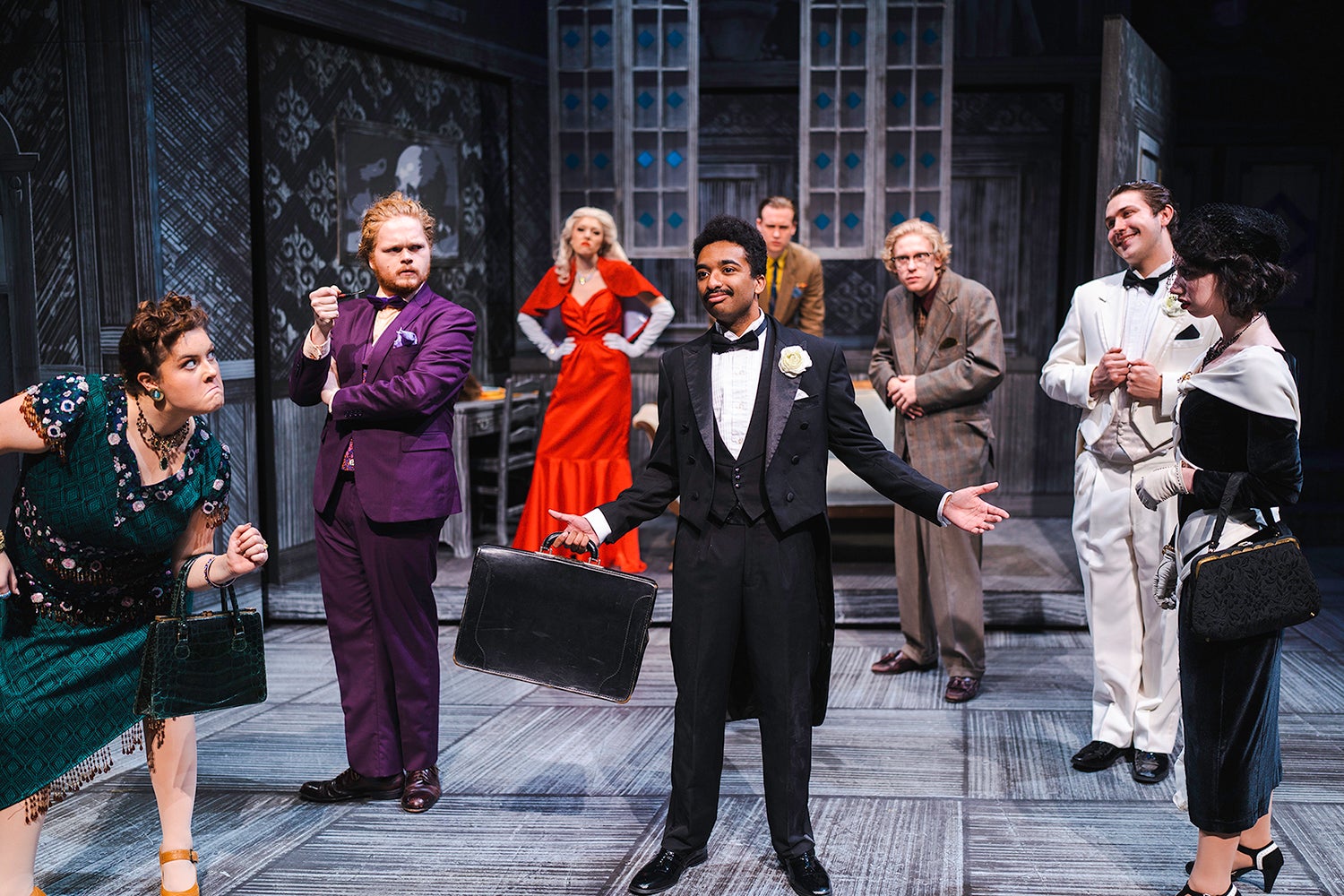
Set in the 17th century, “Or,” takes place over mostly one night in the life of Aphra Behn (1640-1689), a poet, spy and soon-to-be first professional female playwright, as she tries to finish writing a play as she parries the advances of King Charles II, rubs elbows with a celebrated actress, and tests wits with a former spy colleague, in this door-slamming farce.
“What makes this kind of cool is it will be our period show of the year,” Howard said. “So, that gives the opportunity for the student designers to really explore doing something that we would not normally do. We always support our student productions, but this time it’s full on. They have full access to the shops of technical director and carpenters, and scenic artists and costume shop manager and cutters and drapers and stitchers.”
On Feb. 23, “By the Way, Meet Vera Stark,” by two-time Pulitzer Prize winner Lynn Nottage, will take over Will Theatre. Based on the story of actress Theresa Harris, “Vera Stark” follows the life of a Black maid, Gloria Mitchell, as she goes from budding actress in 1930s Hollywood to a fading star trying to hold on to her career. The play draws on screwball comedies of the era to provide an irreverent look at racial stereotypes in Hollywood.
The play will be directed by Assistant Professor Rachel Walshe, who is directing another Nottage play, “Sweat,” at the Gamm Theatre in Warwick. “Lynn Nottage’s work is intensely relevant and human. It’s political but it’s always done in a very wily comic way,” she said. “If you get to work on a Lynn Nottage play, that is, in and of itself, a really great season. As faculty members, our job is to give students a really diverse experience as it relates to the type of plays and the type of styles they work on while always being in the hands of excellent writers.”
The season closes in the spring with the annual musical – the Tony Award-winning and Academy Award-nominated “Into the Woods,” Stephen Sondheim and James Lapine’s classic reworking of popular Brothers Grimm fairytales. The play, directed by URI lecturer Tracy Liz Miller, opens April 20.
The musical centers on the quest by a baker and his wife to begin a family. But they’re stymied by a witch’s curse. To cancel the curse, they must filch Little Red Riding Hood’s cape, a lock of Rapunzel’s hair, Cinderella’s golden slippers, and the cow belonging to Jack (of Jack and the Beanstalk).
“Anytime we produce Steven Sondheim is very exciting,” said Howard. “His work is intellectual, it’s smart and it’s always important and always resonates. It’s some of the most complex musical theater to work on.”
Sondheim has been a popular go-to musical for the department’s year-end show, probably because Howard and former chair Paula McGlasson are big fans. URI last produced “Into the Woods” in 2004 – when Howard designed costumes and played the baker. (He still sings the score in the shower every day, he said.)
“I am incredibly sentimental about that experience,” he said. “It was really important for me and it changed how I worked with students in a lot of ways. It really hit home how invested and how hard working our students are. I’m really looking forward to the students being able to hopefully share the experience that I had with it.”
For a full list of show dates and times, go to the 2022-23 season webpage. Tickets for all the season’s shows go on sale online on Sept. 5. To buy tickets online and see up-to-date COVID-19 guidelines, click here. Tickets may also be purchased in person starting Sept. 26 by phone at (401) 874-5843 or in person at Room 101H in the Fine Arts Center, 105 Upper College Road.